This week we presented our final design report and discussed the culmination of our work for the past two semesters.
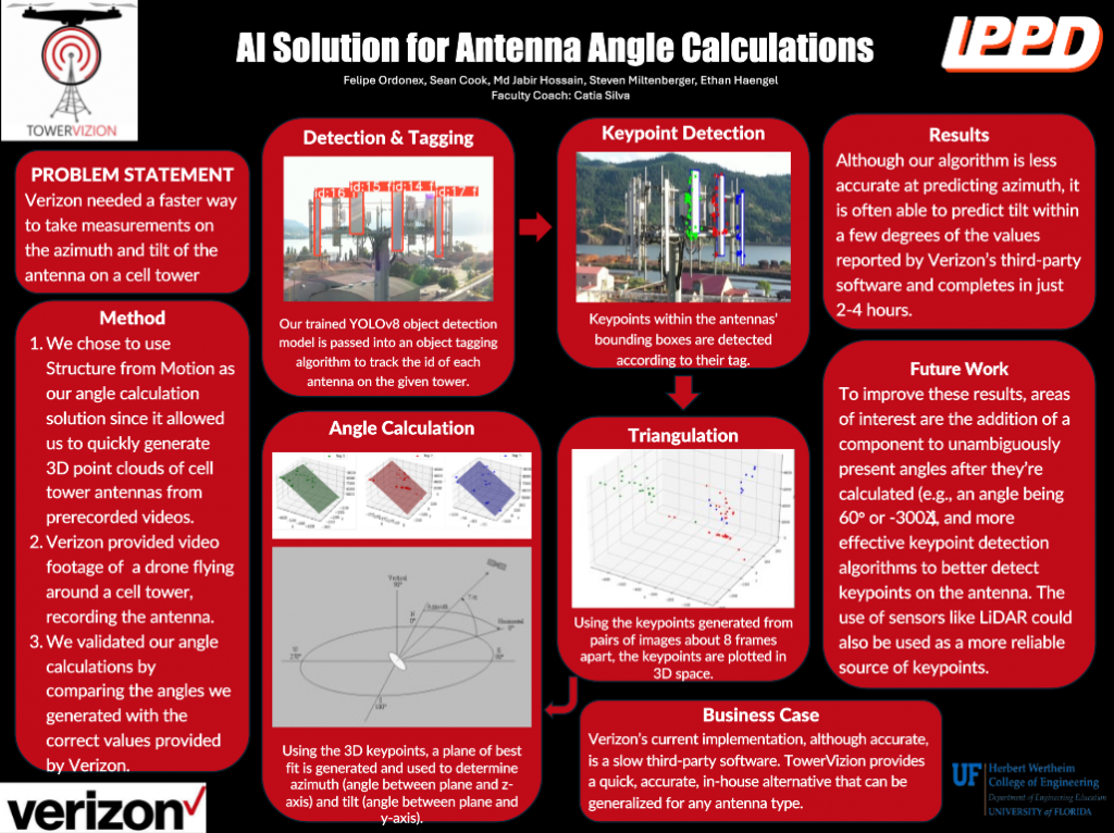
Poster presented at FDR showcase
Overall, the presentation went quite well. Though our liaison was unable to attend, we believe that we were able to accurately portray the potential of our process, explain what was promising, and discuss what can be improved and how.
Video presentation for our project
It was very interesting to discuss our project and the IPPD program with people who weren’t familiar with it before, and was exciting to see the final products presented by all the other teams.
Overall, in spite of the challenges, we are proud of the final product we were able to design, and the experience in tackling a real-world problem will be a vital development in our careers as engineers. Thank you to all the instructors and staff that made this program possible, and special thanks to our coach, Catia Silva for helping us throughout the project.
Throughout the past several weeks, each of us have been working on a different approach to refining the algorithm, so this week we focused on integrating these different approaches into one final pipeline.
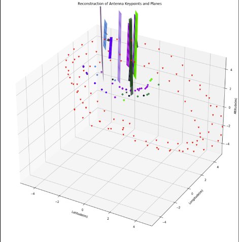
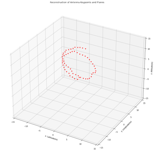
3D Reconstruction generated by final pipeline
Overall, our final estimates for tilt were relatively close to the truth values provided by Verizon. Although the error was more than what would be ideal, our project’s purpose is ultimately to provide a proof of concept that engineers at Verizon could expand upon with more resources.
Although estimates for azimuth were further from the truth values, however we noticed that the predictions were groups together in the same groups as the true antennas. We believe that the reason for this is less with the data itself, and more how that data is presented. Our algorithm loses the information of which direction of the plane of best fit corresponds to the front of the antenna, causing there to be multiple ways to calculate the azimuth of a single plane. So planes with similar angles all get calculated the same way, but if they become too different, our algorithm uses a different calculation.
Ultimately, knowing that Verizon has their own team working on the same problem, but with a different approach, we decided that our time would best be spent improving the aspects of our process that are unique, as opposed to having to spend a large amount of time implementing something that Verizon engineers likely already have.
With our pipeline just needing the finishing touches, the last step is just preparing for FDR!
One of the primary concerns we have had as we inspect and attempt to improve our initial results is that for many frames, our keypoint detection algorithm isn’t able to detect too many keypoints. This creates problems because any inaccuracy in a point’s location will significantly drag the plane of best fit away from what it should be. With more points, any inaccurate points are likely to be diluted, allowing for a more accurate calculation.
To address this, we experimented with a variety of different other keypoint detection algorithms implemented by opencv to observe whether any perform better for our use-case. We also tried using the bounding boxes themselves as keypoints, using the corners and centerpoints of lines between the corners as keypoints.
Results of SIFT keypoint detection
Results of KAZE keypoint detection
Results of AKAZE keypoint detection
We then combined the results, appending the results of multiple algorithms into the list.
Results of several keypoint detection algorithms
While there are still some antennas that are comparatively lacking in keypoints, over the course of several images from the video, we hope that they will all be able to gather a significant number of keypoints.
As be approach the final weeks of the project, we’re getting initial results and need to begin diagnosing how we can improve them. The first step in this is plotting where our algorithm is calculating the camera to be at each frame.
Plot of camera locations at relevant frames during the video.
As you can see, though the plot follows a correct generally circular path, it is at an angle, indicating we need to adjust the initial orientation. Initial testing shows that the initial orientation has a quite significant, and somewhat inconsistent effect on the final angle. This is likely because when the orientation the algorithm believes the camera to be at is different, but not the images, that has a more significant effect on how it calculates the change between the two perspectives for a given point, which results in a significantly different final position.
Using the orientation data from the metadata doesn’t seem to fix the issue, so we will likely need to experiment with the initial orientation parameter just with trial and error.
Following up on our plans from week 7 about using a 3D printed model of a tower in order to validate our results, we are glad to report that the model has been printed, and the process for setting up those tests has begun. We have not yet trained a model on data for the tower, but just for fun (and to see if it wanted to make our lives easier by just working immediately), we decided to run our object detection and tracking algorithm on a video of the tower model:
Video showing object detection and tracking on 3D printed tower analogue
As you can see, it unfortunately is not working perfectly immediately. I’ll emphasize that this is this video is a very different environment compared to the videos that our object detection algorithm was trained on, so the fact that it’s performing this well at all is actually rather surprising. If it can do this well immediately, imagine how well it would do if we actually gave it some applicable training data.
If for whatever reason we really needed to use this model, the biggest problem of it picking up objects in the background, could also be fixed by just setting up piece of paper or something in the background, and just keeping that facing the camera to block out anything in the background.
So while these results aren’t particularly impressive without context, they nonetheless mark an important milestone, and help us to know where we need to focus our efforts in order to keep up with our plans for the future.
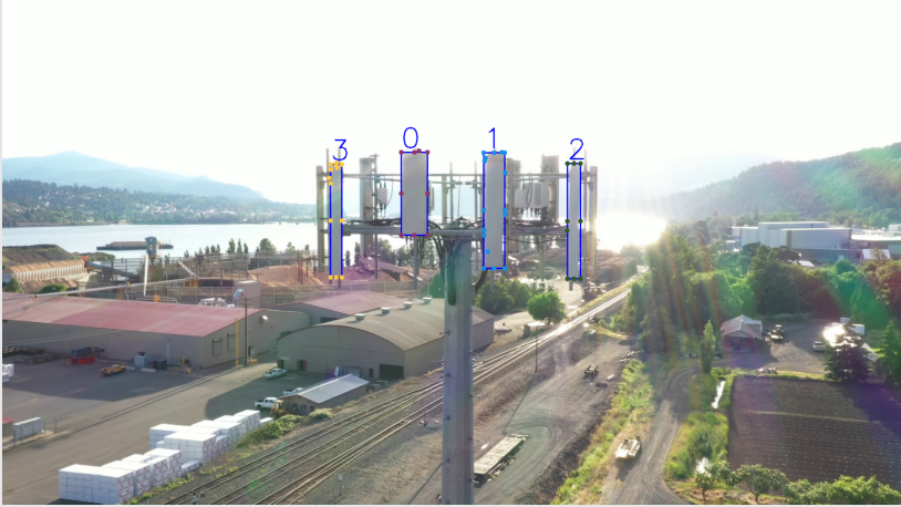
This week, we’re showing off the improvements we made to our object tracking algorithm. If you’ll recall, before, we encountered issues of it reclassifying antennas a lot, resulting in several IDs for the same antenna. Though this is something that could be addressed afterwards, by setting up an algorithm to recognize when multiple IDs correspond to the same antenna, this would be rather complex and take time to do. So instead, we focused on the object detection and tracking algorithm itself, hoping to at the very least reduce the amount of post-processing we would need to do, and here are the results:
As you can see, the algorithm now does a far better job at keeping IDs consistent. There was one period where it lost track of an antenna for some time, and as a result, assigned it a new ID, but that is more likely to be the fault of the object detection algorithm than the object tracking, and is something that can be fixed by adding more training data to that model (which is something either we or Verizon would need to do at some point regardless if this project were to ever be implemented on a large scale).
You may also notice that when the drone makes a complete loop and starts the same antennas in a second loop, that also assigns new IDs. This is something we have planned to address for a while now. If you scroll back to week 8, you’ll see the prototype interface for uploading a video, and under the ‘Description’ field, there is a drop-down with numbers. This is a field for the user to submit the number of antennas on the tower they’re examining. With this information, it should be a simple matter to have our algorithm restart the IDs back to 1 once they reach that maximum value.
Depending on the performance of our angle calculation, and how much data we need from that to get accurate results, we can also simply restrict the input video to only including a single loop of the tower.
Having completed camera calibration last week, we can now begin applying those results to our angle calculation, to hopefully see more accurate results.
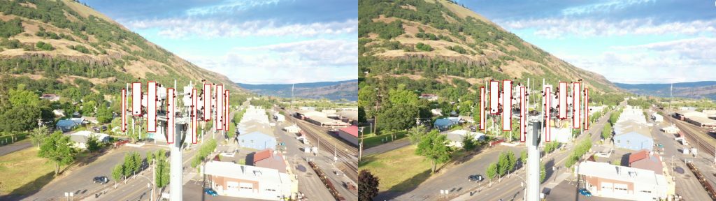
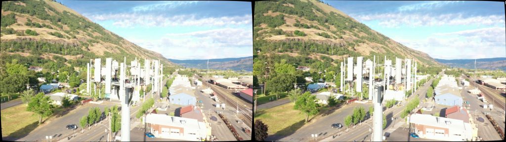
Pair of images before undistortingPair of images after undistorting
Shown above are a pair of images at two different steps in the angle calculation pipeline. Though the difference is not that significant at first glance, you’ll notice that in the second set of images, they are not perfect rectangles, and the frame is slightly curved, particularly near the corners. This is the result of undistorting the images, straightening them out to account for the distortion caused by the camera lens.
Despite the difference not being all that visually significant, in the context of angle calculation, a pixel being slightly off could translate to a difference of several feet, which would then throw off our angle calculation, so in order to ensure our results are as accurate as possible, this is an important and necessary step.
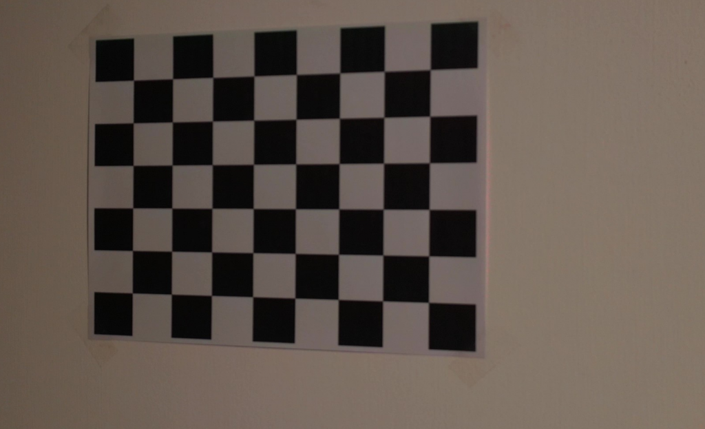
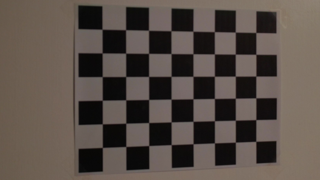
Last week, we received video from Verizon for calibration. This video showed a checkerboard pattern shown below.
Frames from calibration video
Using this video, we can use software to detect the corners, then knowing that the corners should form straight lines with each other, we can calculate how much the lens is distorting the image. By performing this calculation several times across the entire video, we can then get the parameters describing the lens distortion, which we can then apply to our other videos.
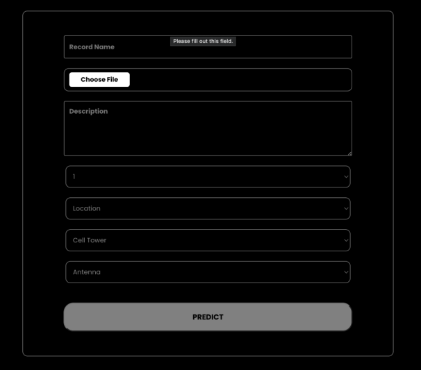
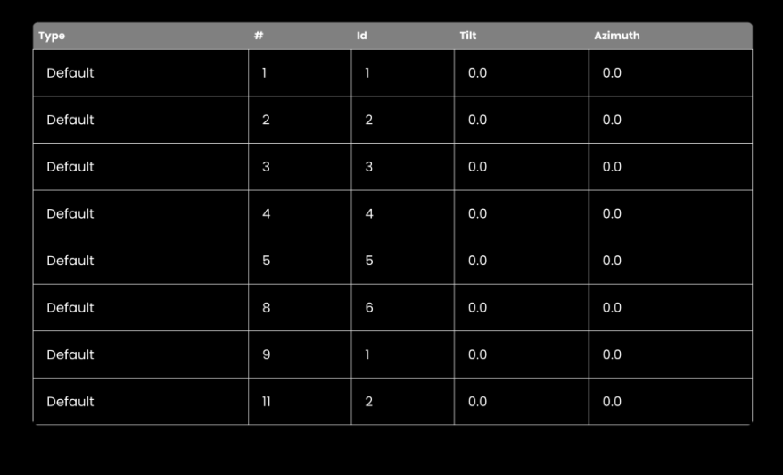
We also created a draft of our basic interface for the project, which will allow users to upload their video and run it through the pipeline.
Upload interface draft, and output table with sample values
This allows us to better plan what information we can request from the user (particularly the number of antennas) and how we want to present our results. It also means once our pipeline is complete, it should simply be a matter of plugging it into the back end, which will aid in testing.
This week, we did our second qualitative review board presentation. The biggest takeaway was ensuring that we have a good way to test and validate our process, in order to both ensure it works, and determine where any issues may be.
We have a couple of approaches to how we can demonstrate the performance of our pipeline. First is, of course, just running the pipeline on the data, and comparing the final values to the true orientation of the antennas. We recently received data from Verizon documenting the orientations of all the antennas in the videos they sent, according to the third-party software they have been using in the past.
But what if our results aren’t immediately perfect? (Hard to imagine, I know.) Well then we’ll need to examine the individual steps of the pipeline to discover where the error is coming from. In most cases, this can be done by examining the intermediary results between these steps. Check how often the object detection is missing the antenna, make sure the 3D tagging isn’t losing track of anything, etc. Where this becomes challenging is in the angle calculations, and particularly in the Structure from Motion portion of the algorithm.
Structure from Motion relies on several parameters which can act as points of failure, and few if any meaningful intermediary results between them. The most notable risks among these are in the camera calibration step. The result of this step is to determine how the intrinsic features of the camera itself (zoom, lens distortion, etc.) are affecting the image so that we can correct for them, and ensure we know exactly where a given pixel refers to. The problem is that we don’t have a drone with which to perform this calibration ourselves. We don’t know how much these parameters might change between cameras even of the same model, or with different camera settings.
We could use a camera we do have, and perform the calibration on that, but since we can’t use that camera to record the cell towers, we wouldn’t be able to demonstrate much besides just that Structure from Motion, as a baseline concept, works (which has already been pretty well proven by countless others).
So if we can’t go to the towers, we’ll simply bring the tower to us.
3D model of tower analogue
In order to test the accuracy of the camera calibration data we’ve been supplied by Verizon, we can run our pipeline using a known camera, taking video of a rough analogue of a cell tower that we designed. The 3D model shown above will be 3D printed, so that if need be, we can see how the pipeline performs using a camera for which we have done the calibration ourselves. Each antenna on the model is at an angle we can measure, allowing us to compare the final results of the pipeline to the true value. This even provides some value over the data supplied by Verizon’s third party company, as that is already an approximation. This allows us to be even more confident that our results are accurate, and within the necessary parameters.
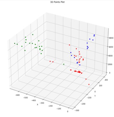
This week, we’ve made quite a bit of progress in integrating our object detection and 3D tagging algorithm with our angle calculation feature. Our project relies on tracking individual antennas, and assigning points as belonging to one antenna or another, in order to then draw a plane of best fit through the points for each antenna, and gathering a series of estimates to average into one conclusion about the orientation of the antenna.
Pointcloud generated for set of 3 antennas, with individual antennas differentiated by color.
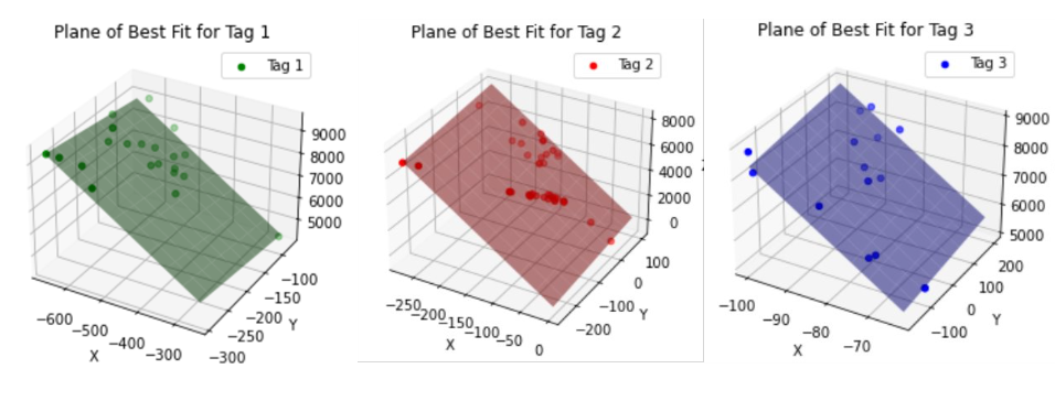
Planes of best fit for each antenna
You may notice that the pointclouds do not currently resemble antennas. This is because we still need to fine-tune the margin around the bounding box with regards to what points to consider to be part of the antenna.
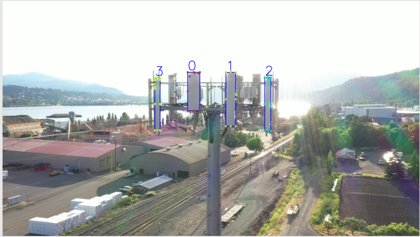
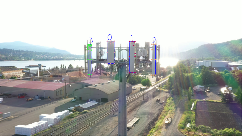
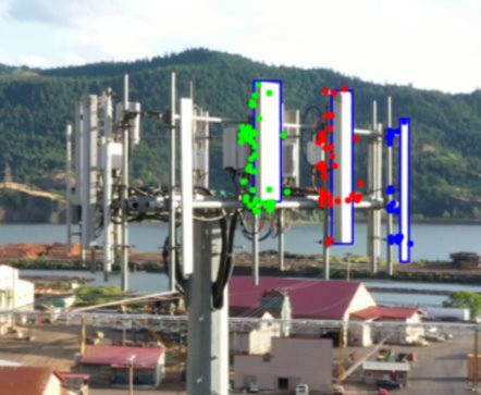
Image showing color-coded key points assigned by the algorithm
We anticipate that many of the keypoints we will use to detect the antenna position will be around the edges of the antenna, as the central portion of the antenna is a consistent texture and appearance, which is difficult for keypoint detection to use. So to ensure that we are getting all the keypoints we can, we need to add a slight margin around the bounding box that will still consider those points to be part of the antenna. That way, even if the bounding box is slightly too small, or barely excludes an edge, we will not miss out on data.
The drawback of this is the results above. With a margin that’s too large, the algorithm will include keypoints for the tower behind the antenna, which throw off our results.
Although it still needs improvement, this integration is nonetheless a marker of significant progress, and brings us one step closer to a complete pipeline.