Author: Will McCoy

I appologize for my deficiency of posts this month. In my experience, the end of October is one of the busiest times of the fall semester, and I was preoccupied with other work. I hope to make up for this with a longer post today; I hope you enjoy.

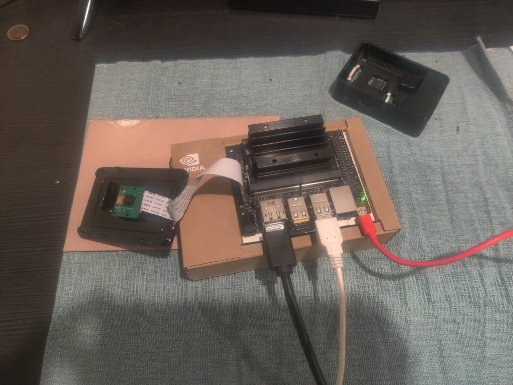
Embedded cameras typically use MIPI CSI, which physically looks like a ribbon cable connecting the camera to the single board computer. My first exposure to this interface was several years ago, when I got my hands on the Raspberry Pi Compute Module 1. I plugged it into my Raspberry Pi (Model 2 B+ I think), an it worked like a charm. A few years later, I purchased an Arduino MKR Vidor 4000, an Arduino board which also features an Altera Cyclone V FPGA. This board also has a MIPI CSI connector, and an (micro) HDMI output. One of the demo projects for this board involved using a MIPI CSI camera and streaming the output to HDMI. I figured I would give it a shot, so I uploaded the code to my board and plugged in my Raspberry Pi Compute Module 1. I expected this to fail due to camera incompatibility; however, it surprisingly worked, and I saw an image on the monitor. This led me to believe that all MIPI CSI cameras, sort of like USB webcams, were generally compatible with each other, as I had plugged in a random camera and it just worked. What were the odds that I just happened to plug in the exact camera the sample code was designed for? 

I specify my history with embedded cameras because I would like to contextualize my error within the scope of my previous experience. Because of this experience, I have gone through this project with the assumption that all MIPI CSI cameras are interoperable. Therefore, I have just been evaluating cameras by their performance specifications, without any consideration as to if they were compatible with the other hardware in the system. Therefore, I was alarmed to find out today that the Jetson Nano only natively supports MIPI CSI cameras based on the IMX219 or IMX477 image sensors; this is because NVIDIA has only officially released drivers for these sensors. Upon discovering this, I was immediately confused, so I looked into why the MKR Vidor camera code worked. Sure enough, the OV5647 image sensor that is in the Raspberry Pi Camera Module 1 just happens to be the exact image sensor required by the MKR Vidor code. What a coincidence! In reality this was probably a deliberate design choice by the Vidor programmers, because they probably assumed the Raspberry Pi Camera Module 1 is the most common MIPI CSI camera for hobbyists, and therefore chose to target it. Nonetheless, this frustrating circumstance has left me misinformed throughout my camera selection process, so its back to the drawing board for now. 

With this in mind, there are several directions to go from here. First, I could just accep the IMX219 limitations, and just use the Raspberry Pi Camera Module 2. Unfortunately, this sensor has less resolution than does the IMX708 in the Raspberry Pi Camera Module 3, which is the camera we are currently considering; this translates directly into a shorter vehicle detection range. Another option is to write my own driver for the IMX708 sensor; I’m still a young and ambitions engineer, so I naively am up for the task. On one hand, NVIDIA’s source code for the IMX219 camera sensor is open source, so I wouldn’t have to start from scratch; I anticipate that the protocols for the two image sensors are sufficiently similar that I could just adapt one into the other. On the other hand, perhaps I should be more realistic, as writing Linux kernel drivers is no easy feat, and I am probably overestimating my abilities. The final option I’ve identified is one provided by ArduCam. They have a product, called JetVariety, which uses their custom hardware and driver, to allow pretty much any MIPI CSI image sensor to be used on the Jetson Nano. The only drawback with this is the added cost, which may prove unviable on our limited budget. 

My current plan is to revisit the math on the range of the Raspberry Pi Camera Module 2. If it turns out that I can actually achieve a larger range, then we can get away with this camera. If not, I’m very tempted to try to adapt the driver for the Raspberry Pi Camera Module 3. If that also fails, we will just be left with the JetVariety solution, though I’d prefer that be a last resort.

The key takeaway of this experience is to always check your assumptions. I generally believe that “things don’t work,” because they often just don’t. However, I should be more cognisant that coincidences like this can still happen, which can give the illusion of things just working. In the future, I will make an effort to better validate my assumptions.

Author: Will McCoy

After considering the budget constraints from the previous week, I focused in on one of the most expensive subcomponents: the camera array. I realized that we could reduce costs if we designed and fabricated the array by ourselves, instead of buying COTS cameras and connecting them together. Through my research this week and last week, I have become familiar enough with cameras to know that their core component is the image sensor, so I figured I would identify the image sensors used in common commercial embedded cameras. I found that many use sensors from OmniVision, such as the OV4689, the OV5640 (Adafruit Camera Breakout), and the OV5647 (Raspberry Pi Camera Module 1). However, newer versions of the Raspberry Pi Camera Modules use sensors from Sony, such as the IMX219 (Raspberry Pi Camera Module 2) and the IMX708 (Raspberry Pi Camera Module 3). I feel like this gives a good basis for investigating and evaluating other sensors, though it is very possible that we may use one of these in our design.

Once we identify the sensors, it will be important to determine how to best arrange them. As seen in my last post, I created a graphic to visualize the overlapping FOVs (fields of vision) in a circular camera array. Making this graphic was time-consuming, yet would be important for evaluating all future camera arrays under consideration. Therefore, this week I automated graphic-generation process; I used SFML to create an interactive environment to explore the array FOVs. Seen below is a screenshot of the output for a circular array of cameras. It should be noted that any 2D configuration can be evaluated with ease using this technique.

Author: Will McCoy

This week we had our first meeting with our Engineering Liaisons at FPL. I’m very glad we were able to do this, because it allowed us to get some of our questions answered. However, an interesting constraint came out of this meeting which will radically change our final design; instead of having the $750-$1500 budget specified in the initial FPL Scope of Work, our sensor solution should end up costing less than $400. Additionally, our sensor should be able to log data about the vehicles it is tracking. These two factors put us in a bit of a pickle. Some baseline research indicates that edge processing systems cost at minimum $100, a camera array would cost at minimum $120, and that LiDARs cost at minimum $90. This leaves us with only $90 for the rest of the project, which may not be feasible. Additionally, there do not seem to be any LiDAR systems that a IP 67 rated and cost under $400. A cheaper solution would be to use 1D sensors, such as RaDAR or LiDAR sensors which only report distances. However, these would not be able to differentiate cars, and therefore would not give meaningful data to log. We will need to be very careful to reconcile these constraints in this project; hopefully it will be possible.

I also spent time this week researching computer vision, which is a field in computation dedicated to extracting information from images. To do this, I read the first chapter of Multiple View Geometry in Computer Vision, a textbook by Hartley and Zisserman. This chapter seemed to summarize the whole book, and thus there was a lot of information to go over. However, now that I know what I don’t know, I should be better able to fill in the gaps. One key takeaway was that, given knowledge about the configuration and properties of two cameras, a 2D point captured by both cameras can be transformed back into a 3D point in the original scene. This principle, called binocular vision, is how the human eye works. Using this principle, I came up with a preliminary design of a camera array, which shows how all points a certain distance from the array can be identified in 3D space (relative to the camera array). This can be seen below.

Author: Will McCoy

I’m happy to report that I am officially the Web-Master of the Road Watch team. When I was reviewing the roles, this one stuck out to me because of my hobby in maintaining a personal website (https://willmccoy.xyz) and my experience with Git. The other role that caught my attention was Team Leader; I have had past positive leadership experiences, mostly in High School when I did Boy Scouts and played baseball. My only concern was that I may not devote enough time to the role because of all my other classes. However, my team decided to divide that position evenly among all team members by periodically rotating it, so I will be the leader eventually.

This week I was introduced to tracking requirements and specifications. Essentially, a requirement is a qualitative description of an aspect of a product, and a specification is a quantitative metric which supports a requirement. Every requirement must have some associated specifications. What I thought was most interesting about this system is that every requirement and specification are given a unique identifying number, so that none are lost or forgotten. This immediately reminded me of relational databases, which also use keys (unique numbers) to identify entries and store the relationships (associations) between them; in fact, many professional Product Requirement Software programs use relational databases to manage requirements and specifications.

In my past work experience, my management’s expectations about projects would change over time. Therefore, I wanted to make a robust system for managing our group’s requirements and specifications, so that when the sponsor inevitably requests a new feature everything can be recorded in an organized way. I spent a few hours in Excel creating what is essentially a bare bones relational database, which records the requirements and specifications, and automatically computes the House of Quality and Technical Performance Measures (TPMs). I have noticed in some of my previous projects that features are often lost when tracking is disorganized, and I hope with this system to avoid that for Road Watch.